← News

Reporte Evaluación 1

Este reporte realiza un análisis de la Evaluación 1 sobre la Unidad 1: Inferencia estadística

Pauta y recorrecciones

La pauta de evaluación se puede revisar aquí

Solicitudes de recorrección

• Enviar correo a apoyo docente Gabriel Cortés, gabriel.cortes@uchile.cl, quien estará coordinando estas solicitudes
• En el correo:
  • mencionar pregunta a corregir
  • argumento y puntaje esperado
  • foto de la pregunta

Solicitudes hasta el Jueves 1 de Octubre 23:59, las solicitudes se responderán en un plazo máximo el miércoles 7 de Octubre.

Librerías, datos y ajustes

pacman::p_load(tidyverse, sjmisc, sjPlot, kableExtra, sjlabelled, readxl, janitor, here)

Generación de la base de datos

Se unen (por RUT) los puntajes por pregunta y la nota (columna “Nota + bonus”) con la asistencia descargada desde U-Cursos.

rut_lista <- read_excel(here("news/data/notas.xls")) %>%
  clean_names() %>%
  pull(rut)

asistencia <- read_excel(here("news/data/asistencia.xls"), .name_repair = "minimal")
asistencia <- asistencia[, 1:4] %>%
  set_names(c("n", "persona", "rut", "asistencia")) %>%
  mutate(asistencia = parse_number(asistencia)) %>%  # "67%" -> 67
  select(rut, asistencia)

puntajes <- read_excel(here("news/data/Puntajes prueba 1.xlsx"), .name_repair = "minimal")
names(puntajes) <- c("n", "persona", "rut", "corrector", "forma", "p1a", "p1b", "p1c",
                     "p2a", "p2b", "p2c", "p2d", "bonus", "puntaje", "nota_puntajes", "nota_bonus")
puntajes <- puntajes %>%
  mutate(across(c(p1a:puntaje), ~ as.numeric(str_replace(as.character(.x), ",", "."))),  # p1c trae comas decimales
         forma = if_else(forma %in% c("A", "B"), forma, NA_character_)) %>%
  # se adaptan las preguntas 2 de la forma B a la forma A: 2aB = 2bA, 2bB = 2cA, 2cB = 2dA, 2dB = 2aA
  mutate(p2a_b = p2a, p2b_b = p2b, p2c_b = p2c, p2d_b = p2d,
         p2a = if_else(forma == "B", p2d_b, p2a),
         p2b = if_else(forma == "B", p2a_b, p2b),
         p2c = if_else(forma == "B", p2b_b, p2c),
         p2d = if_else(forma == "B", p2c_b, p2d)) %>%
  select(-ends_with("_b")) %>%
  # quienes no rindieron tienen todo vacío (puntaje 0 / nota 1 solo por defecto)
  mutate(across(c(p1a:puntaje), ~ if_else(is.na(p1a), NA_real_, .x))) %>%
  select(rut, persona, corrector, forma, p1a:p2d, bonus, puntaje, nota = nota_bonus) %>%  # nota = nota + bonus
  mutate(nota = floor(nota * 10 + 0.5 + 1e-9) / 10)  # redondeo a 1 decimal (mitad hacia arriba), como U-Cursos

prueba1 <- puntajes %>%
  left_join(asistencia, by = "rut")

stopifnot(nrow(prueba1) == length(rut_lista), !anyDuplicated(prueba1$rut))

Un caso (corrector JC) trae en forma el valor “2.0” (error de digitación); queda como forma perdida.

Etiquetados

prueba1 <- prueba1 %>%
  set_label(c(persona = "Estudiante", corrector = "Corrector/a", forma = "Forma de la prueba",
              p1a = "1a: Hipótesis", p1b = "1b: Valor t", p1c = "1c: Intervalo",
              p2a = "2a: 2 muestras", p2b = "2b: Intervalos", p2c = "2c: Alfa y p", p2d = "2d: Hijos",
              bonus = "Bonus", puntaje = "Puntaje total (con bonus)",
              nota = "Nota final", asistencia = "Asistencia (%)")[names(.)])

Sin nota (no rindieron la prueba): 21. Sin registro de asistencia: 2.

Descriptivos

Tabla descriptiva

prueba1 %>% select(p1a:p2d, bonus, puntaje, nota, asistencia) %>% descr(show = c("label","range", "mean", "sd", "n")) %>% kable(.,"markdown", digits=2)

	var	label	n	mean	sd	range
4	p1a	1a: Hipótesis	87	1.16	0.90	3 (0-3)
5	p1b	1b: Valor t	87	2.43	1.38	4 (0-4)
6	p1c	1c: Intervalo	87	0.68	0.70	2 (0-2)
7	p2a	2a: 2 muestras	87	0.21	0.41	1 (0-1)
8	p2b	2b: Intervalos	87	0.54	0.50	1 (0-1)
9	p2c	2c: Alfa y p	87	0.32	0.47	1 (0-1)
10	p2d	2d: Hijos	87	0.34	0.48	1 (0-1)
2	bonus	Bonus	87	0.31	0.23	0.5 (0-0.5)
11	puntaje	Puntaje total (con bonus)	87	5.99	2.82	11.5 (0-11.5)
3	nota	Nota final	87	4.16	1.46	6 (1-7)
1	asistencia	Asistencia (%)	106	74.63	20.65	75 (25-100)

Ajuste entre formas

• Pregunta 2: las preguntas 2 de la forma B se adaptaron a la forma A, según esta equivalencia: 2a B = 2b A, 2b B = 2c A, 2c B = 2d A y 2d B = 2a A. Las etiquetas de la tabla corresponden a la forma A.
• Pregunta 1: en la forma A se refiere a una hipótesis no direccional; en la forma B, a una hipótesis direccional.

Gráficos descriptivos

plot_frq(data = prueba1$nota, type = "hist", show.mean = T)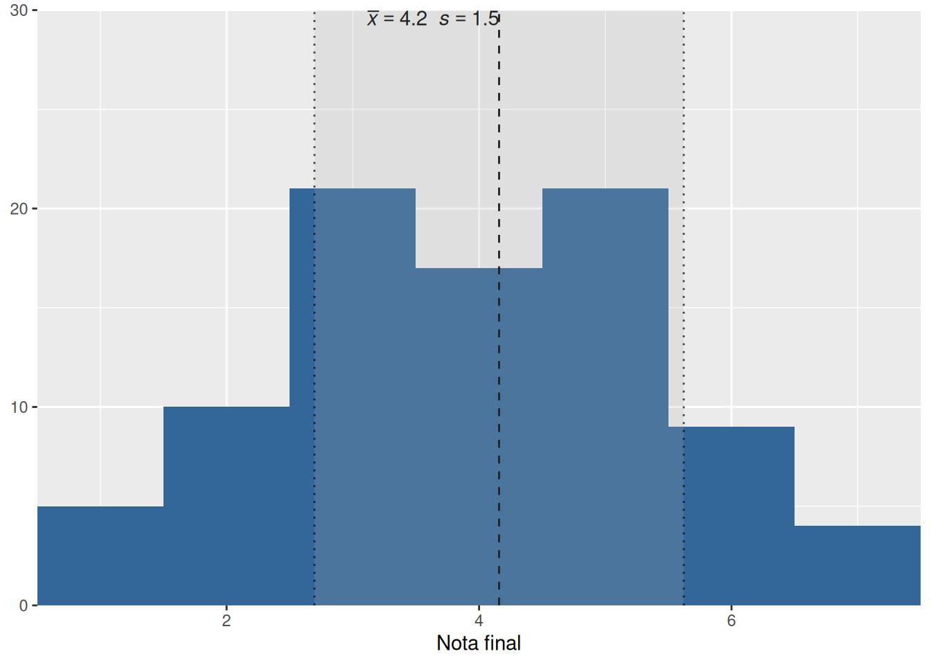

prueba1 %>%
  filter(!is.na(nota)) %>%
  mutate(notas_cat = cut(nota, breaks = c(-Inf, 3.95, 4.95, 5.95, Inf),
                         labels = c("Menor a 4.0", "4.0-4.9", "5.0-5.9", "6.0-7.0"))) %>%
  count(notas_cat) %>%
  mutate(pct = n / sum(n)) %>%
  ggplot(aes(x = n, y = fct_rev(notas_cat))) +
  geom_col(fill = "steelblue") +
  geom_text(aes(label = paste0(n, " (", round(pct * 100, 1), "%)")), hjust = -0.1, size = 6) +
  scale_x_continuous(expand = expansion(mult = c(0, 0.35))) +
  labs(title = "Rangos de notas en Evaluación 1", x = "Estudiantes", y = NULL) +
  theme_minimal(base_size = 16) +
  theme(plot.title = element_text(face = "bold", hjust = 0.5),
        axis.text.y = element_text(size = 18),
        axis.text.x = element_text(size = 14),
        axis.title = element_text(size = 16))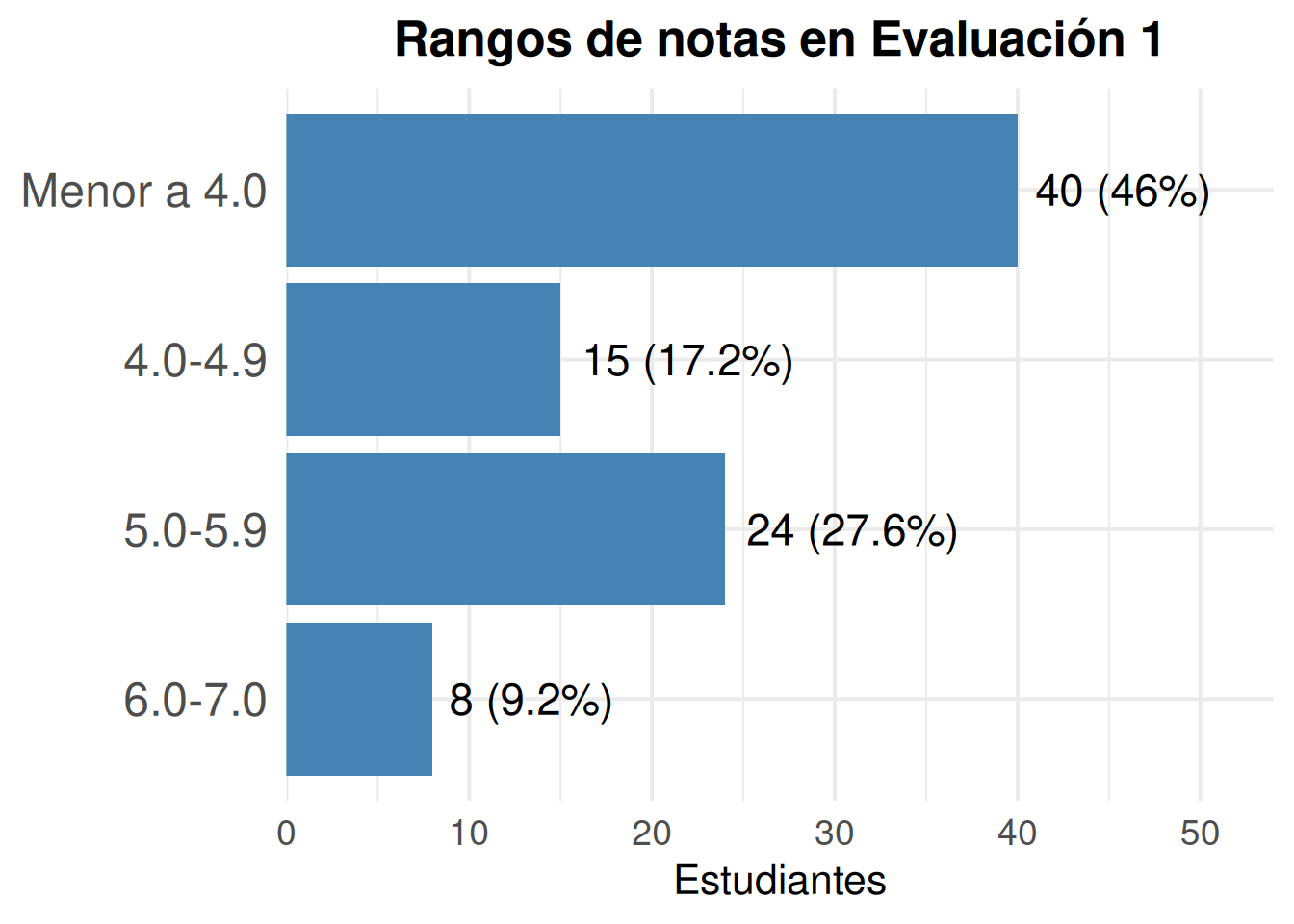

Asociación entre asistencia y nota

r <- cor(prueba1$asistencia, prueba1$nota, use = "complete.obs")

ggplot(prueba1, aes(x = asistencia, y = nota)) + 
  geom_jitter(width = 0.2, color = "red", size = 4) + 
  labs(title = paste0("Relación entre asistencia y notas en Evaluación 1 (r=", round(r, 2), ")"),
       x = "Asistencia (%)", y = "Nota") + 
  theme(axis.title = element_text(size = 12),
        axis.text = element_text(size = 12),
        aspect.ratio = 1/1.5,
        plot.title = element_text(size = 12, face = "bold", hjust = 0.5)) +
  scale_x_continuous(breaks = seq(0, 100, by = 10), limits = c(0, 100)) +
  scale_y_continuous(breaks = 1:7, limits = c(1, 7)) +
  geom_vline(xintercept = 50, linetype = "dashed") +
  geom_hline(yintercept = 4, linetype = "dashed")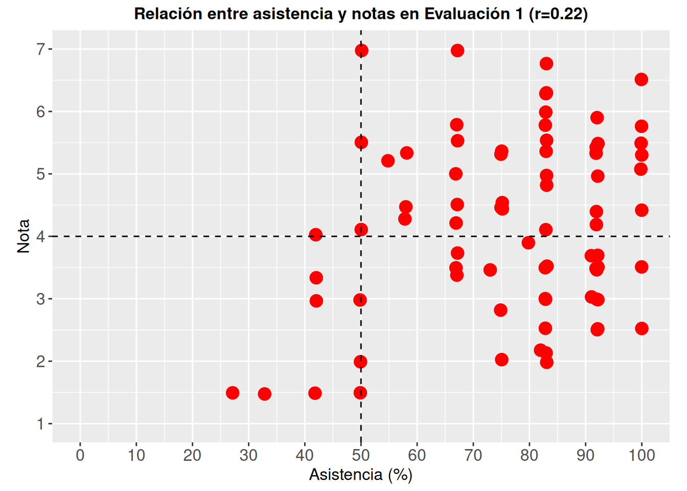

Cuadrantes según nota (4.0) y asistencia (50%)

cuadrantes <- prueba1 %>%
  filter(!is.na(nota), !is.na(asistencia)) %>%
  mutate(cuadrante = case_when(
    asistencia >= 50 & nota >= 4 ~ "Asistencia alta y nota ≥ 4.0",
    asistencia >= 50 & nota <  4 ~ "Asistencia alta y nota < 4.0",
    asistencia <  50 & nota >= 4 ~ "Asistencia baja y nota ≥ 4.0",
    asistencia <  50 & nota <  4 ~ "Asistencia baja y nota < 4.0")) %>%
  group_by(cuadrante) %>%
  summarise(n = n(), nota_media = mean(nota)) %>%
  mutate(pct = n / sum(n) * 100)

cuadrantes %>%
  transmute(Cuadrante = cuadrante, N = n, `% estudiantes` = pct, `Nota promedio` = nota_media) %>%
  kable(digits = 1)

Cuadrante	N	% estudiantes	Nota promedio
Asistencia alta y nota < 4.0	35	40.7	2.9
Asistencia alta y nota ≥ 4.0	45	52.3	5.3
Asistencia baja y nota < 4.0	5	5.8	2.2
Asistencia baja y nota ≥ 4.0	1	1.2	4.0

q <- function(x) filter(cuadrantes, cuadrante == x)

Considerando a los 86 estudiantes con nota y asistencia, y usando como puntos de corte la nota 4.0 y el 50% de asistencia:

• 52.3% (n = 45) tiene asistencia igual o superior a 50% y nota igual o superior a 4.0; su nota promedio es 5.33.
• 40.7% (n = 35) tiene asistencia igual o superior a 50% y nota inferior a 4.0; su nota promedio es 2.93.
• 1.2% (n = 1) tiene asistencia inferior a 50% y nota igual o superior a 4.0; su nota promedio es 4.
• 5.8% (n = 5) tiene asistencia inferior a 50% y nota inferior a 4.0; su nota promedio es 2.16.

Preguntas y asociaciones

tab_corr(select(prueba1, p1a:p2d, puntaje, nota, asistencia),
         triangle = "lower")

	1a: Hipótesis	1b: Valor t	1c: Intervalo	2a: 2 muestras	2b: Intervalos	2c: Alfa y p	2d: Hijos	Puntaje total (con bonus)	Nota final	Asistencia (%)
1a: Hipótesis
1b: Valor t	0.251*
1c: Intervalo	0.314**	0.561***
2a: 2 muestras	0.104	0.244*	0.166
2b: Intervalos	0.335**	0.218*	0.182	0.276*
2c: Alfa y p	-0.146	-0.250*	-0.138	0.154	0.184
2d: Hijos	0.095	0.141	0.065	0.140	0.353***	0.187
Puntaje total (con bonus)	0.597***	0.769***	0.673***	0.446***	0.567***	0.067	0.402***
Nota final	0.596***	0.758***	0.673***	0.440***	0.558***	0.079	0.390***	0.997***
Asistencia (%)	0.329**	-0.024	0.125	0.029	0.262*	0.059	-0.014	0.209	0.224*
Computed correlation used pearson-method with listwise-deletion.

Consistencia interna

pacman::p_load(psych)

preguntas <- prueba1 %>% select(p1a:p2d)
psych::alpha(preguntas)$total$raw_alpha

Some items ( p2c ) were negatively correlated with the first principal component and 
probably should be reversed.  
To do this, run the function again with the 'check.keys=TRUE' option

[1] 0.5402977